
| 일 | 월 | 화 | 수 | 목 | 금 | 토 |
|---|---|---|---|---|---|---|
| 1 | 2 | 3 | ||||
| 4 | 5 | 6 | 7 | 8 | 9 | 10 |
| 11 | 12 | 13 | 14 | 15 | 16 | 17 |
| 18 | 19 | 20 | 21 | 22 | 23 | 24 |
| 25 | 26 | 27 | 28 | 29 | 30 | 31 |
Tags
- Slicing
- pandas filter
- matplotlib
- INSERT
- 조합
- Machine Learning
- 등차수열
- 재귀함수
- 자료구조
- plt
- 순열
- maplotlib
- 문제풀이
- barh
- 스터디노트
- MacOS
- pandas
- Folium
- SQL
- 기계학습
- 머신러닝
- 통계학
- tree.fit
- 파이썬
- pandas 메소드
- DataFrame
- python
- 리스트
- 등비수열
- numpy
Archives
- Today
- Total
코딩하는 타코야끼
[스터디 노트] Week12_2일차 [4 ~ 5] - ML 본문
728x90
반응형
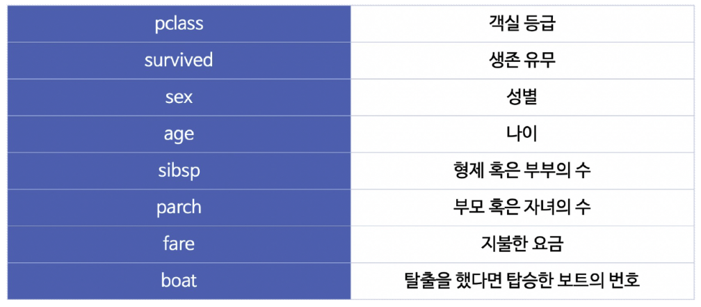
1. 타이타닉 생존자 분석 - EDA
📍 컬럼의 의미
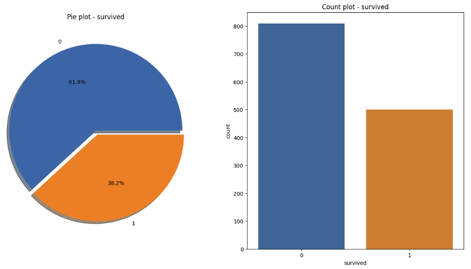
📍 생존 상황
import matplotlib.pyplot as plt
import seaborn as sns
%matplotlib inline

# 데이터 정의
titanic_url = "<https://raw.githubusercontent.com/PinkWink/ML_tutorial/master/dataset/titanic.xls>"
titanic = pd.read_excel(titanic_url)
titanic.head()

# 시각화
f, ax = plt.subplots(1, 2 ,figsize=(16, 8))
titanic["survived"].value_counts().plot.pie(ax=ax[0], autopct="%1.1f%%", shadow=True, explode=[0, 0.05])
ax[0].set_title("Pie plot - survived")
ax[0].set_ylabel("")

sns.countplot(x="survived", data=titanic, ax=ax[1])
ax[1].set_title("Count plot - survived")

plt.show()
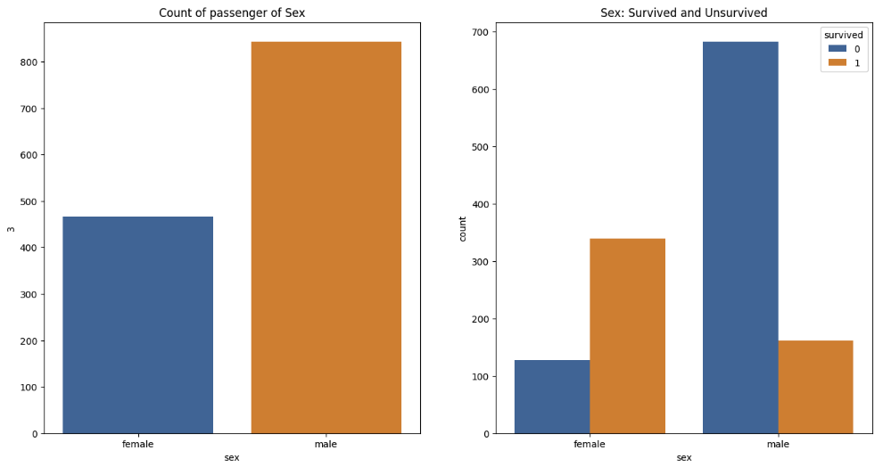
📍 성별에 따른 생존 상황
f, ax = plt.subplots(1, 2 ,figsize=(16, 8))

sns.countplot(x="sex", data=titanic, ax=ax[0])
ax[0].set_title("Count of passenger of Sex")
ax[0].set_ylabel(3)

sns.countplot(x="sex", hue="survived", data=titanic, ax=ax[1])
ax[1].set_title("Sex: Survived and Unsurvived")

plt.show()
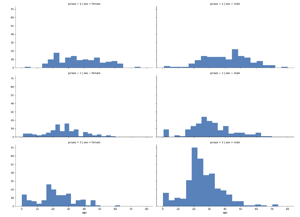
🔌 3등실에는 남성이 많았다, 특히 20대 남성
grid = sns.FacetGrid(titanic, row="pclass", col="sex", height=4, aspect=2)
grid.map(plt.hist, "age", alpha=0.8, bins=20)
grid.add_legend()

plt.show()
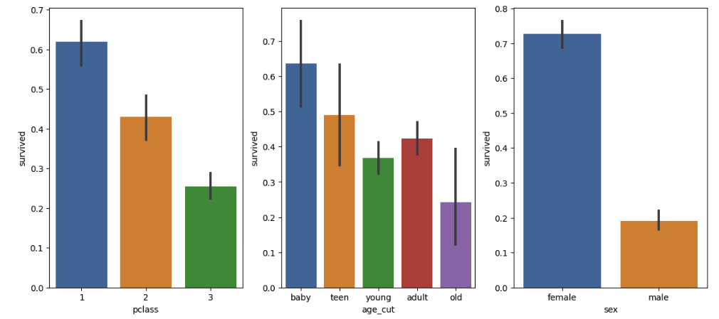
🔌 생존율
plt.figure(figsize=(14, 6))

# 선실 등급별 생존율
plt.subplot(131)
sns.barplot(x="pclass", y="survived", data=titanic)

# 나이별 생존율
plt.subplot(132)
sns.barplot(x="age_cut", y="survived", data=titanic)

# 성별 생존율
plt.subplot(133)
sns.barplot(x="sex", y="survived", data=titanic)

plt.show()
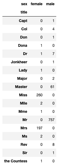
🔌 성별 별로 본 귀족
# 탑승객의 이름에서 신분을 알 수 있다
import re

title = []
for idx, dataset in titanic.iterrows():
    tmp = dataset["name"]
    title.append(re.search('\\,\\s\\w+(\\s\\w+)?\\.', tmp).group()[2:-1])

titanic["title"] = title

pd.crosstab(titanic["title"], titanic["sex"])
🔌 사회적 신분 정리
titanic["title"] = titanic["title"].replace("Mlle", "Miss")
titanic["title"] = titanic["title"].replace("Ms", "Miss")
titanic["title"] = titanic["title"].replace("Mme", "Mrs")

Rare_f = ["Dona", "Dr", "Lady", "the Countess"]
Rare_m = ["Capt", "Col", "Don", "Major", "Rev", "Sir", "Jonkheer", "Master"]

for each in Rare_f:
    titanic["title"] = titanic["title"].replace(each, "Rare_f")

for each in Rare_m:
    titanic["title"] = titanic["title"].replace(each, "Rare_m")

# 평민 남성 -> 귀족 남성 -> 평민 여성 -> 귀족 여성 순서 (생존율)
titanic[["title", "survived"]].groupby(["title"], as_index=False).mean()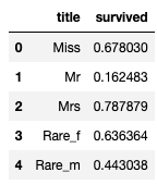
2. 타이타닉 생존자 분석 - 모델 구축
⚡️ 모델 학습
from sklearn.preprocessing import LabelEncoder

le = LabelEncoder()
le.fit(titanic["sex"])
⚡️"sex" 값을 모델을 통해 변환후 "gender"에 반환
titanic["gender"] = le.transform(titanic["sex"])
titanic.head()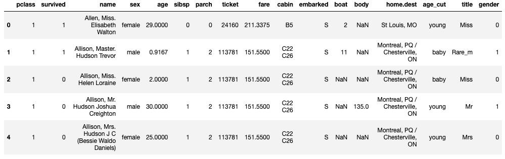
⚡️ 결측치 제거
titanic = titanic[titanic["age"].notnull()]
titanic = titanic[titanic["fare"].notnull()]
titanic.info()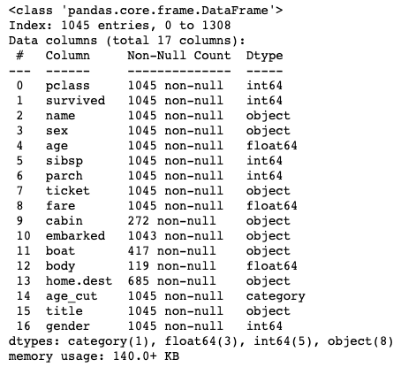
⚡️데이터셋 분리 및 모델 학습
# 데이터셋 분리
from sklearn.tree import DecisionTreeClassifier
from sklearn.model_selection import train_test_split
from sklearn.metrics import accuracy_score

X = titanic[["pclass", "age", "sibsp", "parch", "fare", "gender"]]
y = titanic["survived"]

X_train, X_test, y_train, y_test = train_test_split(X, y,
                                                    test_size=0.2,
                                                   stratify=y,
                                                   random_state=0)

tree = DecisionTreeClassifier(random_state=0)
tree.fit(X_train, y_train)
⚡️ 예측 및 추론
pred = tree.predict(X_test)
print(accuracy_score(y_test, pred))
>>>
0.7368421052631579
⚡️ 오류제거
import warnings
from sklearn.exceptions import DataConversionWarning
warnings.filterwarnings(action='ignore', category=UserWarning)
⚡️ 디카프리오와 윈슬릿의 생존율
dicaprio = np.array([[3, 18, 0, 0, 5, 1]])
winslet = np.array([[1, 16, 1, 1, 100, 0]])

print("Dicaprio: ", tree.predict_proba(dicaprio)[0, 1])
print("Winslet: ", tree.predict_proba(winslet)[0, 1])
>>>
Dicaprio: 0.0
Winslet:  1.0
3. Encoder and Scaler
📍 label encoder
- 목적: 범주형 변수를 숫자로 변환합니다.
- 작동 방식: 각 범주에 고유한 정수를 할당합니다. 예를 들어, ['red', 'green', 'blue']는 [0, 1, 2]로 변환될 수 있습니다.
- 주의점: 이 방법은 명목형 변수에만 적합합니다. 순서형 변수에는 순서가 중요하므로 다른 인코딩 방법을 사용해야 할 수 있습니다.
df = pd.DataFrame({
    "A": ["a", "b", "c", "a", "b"],
    "B": [1, 2, 3, 1, 0]
})
df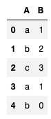
⚡️ 모델 학습 및 변환
from sklearn.preprocessing import LabelEncoder

# 모델 학습
le = LabelEncoder()
le.fit(df["A"])

# 변환
df["transform"] = le.transform(df["A"])
df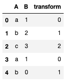
⚡️ 학습과 변환을 동시에 진행
# 학습과 변환을 동시에 진행
le.fit_transform(df["A"]
# 역변환
le.inverse_transform(df["transform"])
>>>
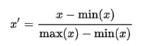
array(['a', 'b', 'c', 'a', 'b'], dtype=object)📍 min-max scaler
- 목적: 데이터를 특정 범위(주로 0과 1 사이)로 조정합니다.
- 특징: 이 방법은 이상치에 민감합니다. 큰 이상치가 있을 경우 스케일링 범위가 왜곡될 수 있습니다.
⚡️ 표준정규분포 식
from sklearn.preprocessing import MinMaxScaler

# 학습
mms = MinMaxScaler()
mms.fit(df)

# 변환
df_mms = mms.transform(d)

# 역변환
mms.inverse_transform(df_mms)

# 학습 및 변환
mms.fit_transform(df)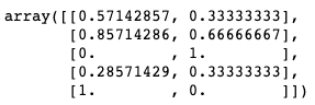
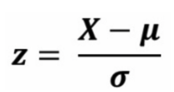
📍 standard scaler
- 목적: 데이터의 평균을 0, 표준 편차를 1로 조정하여 정규화합니다.
- 특징: 이 방법 역시 이상치에 민감합니다. 그러나 많은 머신러닝 알고리즘이 가정하는 정규 분포를 따르는 데이터 형태에 가깝게 만들어줍니다.
⚡️ 표준정규분포
from sklearn.preprocessing import StandardScaler

ss = StandardScaler()
ss.fit(df)

# 케일러가 학습한 각 특성의 평균, 표준편차 값을 반환
ss.mean_, ss.scale_
>>>
(array([9. , 1.4]), array([12.80624847,  1.0198039 ]))
⚡️ 모델 변환
ss.transform(df)
>>>
array([[ 0.07808688, -0.39223227],
       [ 0.85895569,  0.58834841],
       [-1.48365074,  1.56892908],
       [-0.70278193, -0.39223227],
       [ 1.2493901 , -1.37281295]])
⚡️ 모델 역변환
ss.inverse_transform(df_ss)
>>>
array([[ 10.,   1.],
       [ 20.,   2.],
       [-10.,   3.],
       [  0.,   1.],
       [ 25.,   0.]])
⚡️ 모델 학습 변환
ss.fit_transform(df)
>>>
array([[ 0.07808688, -0.39223227],
[ 0.85895569, 0.58834841],
[-1.48365074, 1.56892908],
[-0.70278193, -0.39223227],
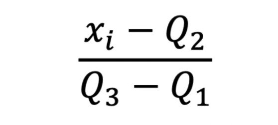
[ 1.2493901 , -1.37281295]])📍 robust scaler
- 목적: 이상치의 영향을 최소화하면서 데이터를 스케일링합니다.
- 특징: 중앙값과 사분위 범위를 사용하여 스케일링하므로 이상치에 덜 민감합니다.
⚡️ 표준정규분포 식
반응형
'zero-base 데이터 취업 스쿨 > 스터디 노트' 카테고리의 다른 글
| [스터디 노트] Week12_3일차 [6 ~ 7] - ML (0) | 2023.10.11 |
|---|---|
| [스터디 노트] Week12_1일차 [1 ~ 3] - ML (1) | 2023.10.10 |
| [스터디 노트] Week10_3일차 [기본] - 통계학 (1) | 2023.09.11 |
| [스터디 노트] Week10_2일차 [기본] - 통계학 (0) | 2023.09.11 |
| [스터디 노트] Week10_1일차 [기본] - 통계학 (2) | 2023.09.11 |
'zero-base 데이터 취업 스쿨/스터디 노트' Related Articles
more


